Examples

1. Equilibrium Plummer sphere

2. Satellite disrupting in an external halo potential

3. Reflex motion of the Sun due to Venus and Jupiter

4. Sample a galpy NFW spherical distribution function

5. Bobbing and oscillating orbit in a galactic disk

6. Galaxy merger

7. Initial conditions from cosmological simulation output

Equilibrium Plummer sphere

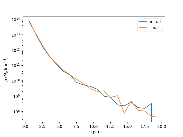
Create an equilibrium Plummer sphere. Evolve for 2 Myr, and demonstrate that it stays in equilibrium by plotting before-and-after density profiles and making a movie of the evolution:

from gravhopper import Simulation, IC
from astropy import units as u
import matplotlib.pyplot as plt
from pynbody.analysis.profile import Profile

# Create and run the simulation
sim = Simulation(dt=5e3*u.yr, eps=0.05*u.pc)
Plummer_IC = IC.Plummer(N=5000, b=1*u.pc, totmass=1e6*u.Msun)
sim.add_IC(Plummer_IC)
sim.run(400)

# Plot density profile before and after
s_IC = sim.pyn_snap(timestep=0)
s_final = sim.pyn_snap()
p_IC = Profile(s_IC, ndim=3, min=0.0001, max=0.02, nbins=20)
p_final = Profile(s_final, ndim=3, min=0.0001, max=0.02, nbins=20)
plt.plot(p_IC['rbins'].in_units('pc'), p_IC['density'], label='initial')
plt.plot(p_final['rbins'].in_units('pc'), p_final['density'], label='final')
plt.yscale('log')
plt.xlabel('r (pc)')
plt.ylabel(f'$\\rho$ (${p_IC["density"].units.latex()}$)')
plt.legend()

# Make a movie of the simulation
sim.movie_particles('Plummer-equilibrium.mp4', unit=u.pc, xlim=[-5,5], ylim=[-5,5])

Satellite disrupting in an external halo potential

Create an equilibrium Hernquist sphere satellite. Put it in an external logarithmic potential on an elliptical orbit and make a movie of it getting tidally disrupted:

from gravhopper import Simulation, IC
from astropy import units as u
from galpy.potential import LogarithmicHaloPotential

# Create and run the simulation
sim = Simulation(dt=5*u.Myr, eps=0.05*u.kpc)
Hernquist_IC = IC.Hernquist(N=5000, a=1*u.kpc, totmass=1e9*u.Msun,
    center_pos=[50,0,0]*u.kpc, center_vel=[0,100,0]*u.km/u.s)
sim.add_IC(Hernquist_IC)
externalpot = LogarithmicHaloPotential(amp=(200*u.km/u.s)**2)
sim.add_external_force(externalpot)
sim.run(400)

# Make a movie of the simulation
sim.movie_particles('satellite-stripping.mp4', timeformat='{0:.0f}')

Reflex motion of the Sun due to Venus and Jupiter

Create a simple Solar System model with the Sun, Venus, and Jupiter. Evolve for about 2 Jovian years and plot the radial velocity of the Sun as seen by an observer in the ecliptic:

from gravhopper import Simulation
from astropy import units as u
import matplotlib.pyplot as plt

# Create and run the simulation
sim = Simulation(dt=10*u.day, eps=0.0001*u.au)
Sun = {'pos':[0, 0, 0]*u.au, 'vel':[0, 0, 0]*u.km/u.s, 'mass':[1]*u.Msun}
Venus = {'pos':[0,107.5e6, 0]*u.km, 'vel':[-35.23, 0, 0]*u.km/u.s, 'mass':[4.87e24]*u.kg}
Jupiter = {'pos':[-816.6e6,0,0]*u.km, 'vel':[0,-12.49,0]*u.km/u.s, 'mass':[1898e24]*u.kg}
sim.add_IC(Sun)
sim.add_IC(Venus)
sim.add_IC(Jupiter)
sim.run(800)

# Plot the Sun's x velocity.
plt.plot(sim.times.to(u.yr), sim.velocities[:,0,0].to(u.m/u.s))
plt.xlabel('t (yr)')
plt.ylabel('v (m/s)')

Sample a galpy NFW spherical distribution function

Create a galpy NFW distribution function and sample it to create a set of equilibrium initial conditions. Demonstrate that it stays in equilibrium by making a movie of the evolution:

from gravhopper import Simulation, IC
from astropy import units as u
from galpy import potential, df
import matplotlib.pyplot as plt

# Set up useful constants
ro = 8. # galpy unit system
vo = 220. # more galpy unit system
rmax = 0.5*u.Mpc
rmax_over_ro = (rmax/(ro*u.kpc)).to(1).value
Nhalo = 5000

# Create the distribution function object and IC from it
NFWpot = potential.NFWPotential(amp=2e11*u.Msun, a=20*u.kpc)
NFWmass = potential.mass(NFWpot, rmax)
potential.turn_physical_off(NFWpot)
NFWdf = df.isotropicNFWdf(pot=NFWpot, rmax=rmax_over_ro)
NFW_IC = IC.from_galpy_df(NFWdf, N=Nhalo, totmass=NFWmass)

# Create and run the simulation
sim = Simulation(dt=10*u.Myr, eps=1*u.kpc)
sim.add_IC(NFW_IC)
sim.run(400)

# Convert time to Gyr and make a movie
sim.times = sim.times.to(u.Gyr)
sim.movie_particles('NFWdf.mp4', timeformat='{0:.2f}', xlim=[-200,200], ylim=[-200,200])

Bobbing and oscillating orbit in a galactic disk

Create an exponential disk in an external NFW potential. Follow the orbit of a particle that is in a not-quite-circular orbit for a few orbital timescales:

from gravhopper import Simulation, IC
from astropy import units as u
from galpy import potential
import matplotlib.pyplot as plt

# Set up an external NFW potential and an exponential disk that uses its rotation curve
NFWpot = potential.NFWPotential(amp=2e11*u.Msun, a=20*u.kpc)
potential.turn_physical_on(NFWpot)
expdisk_IC = IC.expdisk(N=5000, sigma0=100*u.Msun/u.pc**2, Rd=2*u.kpc, z0=0.2*u.kpc, sigmaR_Rd=20*u.km/u.s,
    external_rotcurve=NFWpot.vcirc)
# Create a tracer particle to be particle 0
particle = {'pos':[3.5,0,0]*u.kpc, 'vel':[10,70,10]*u.km/u.s, 'mass':[1]*u.Msun}

# Create and run the simulation
sim = Simulation(dt=2*u.Myr, eps=0.1*u.kpc)
sim.add_IC(particle)
sim.add_IC(expdisk_IC)
sim.add_external_force(NFWpot)
sim.run(500)

# Plot the xy and xz trajectories of the tracer particle
fig = plt.figure(figsize=(10,4))
ax_xy = fig.add_subplot(121, aspect=1.0)
ax_xz = fig.add_subplot(122, aspect=1.0)
ax_xy.plot(sim.positions[:,0,0], sim.positions[:,0,1])
ax_xz.plot(sim.positions[:,0,0], sim.positions[:,0,2])
ax_xy.set_xlabel('x (kpc)')
ax_xy.set_ylabel('y (kpc)')
ax_xz.set_xlabel('x (kpc)')
ax_xz.set_ylabel('z (kpc)')

Galaxy merger

Create two exponential disks with truncated isothermal halos, offset and tilted, and make a movie of just the disk particles and just the dark matter particles. Note that this one takes longer because it has over 40,000 particles, compared to <5,000 in the other examples. This is required to keep the dark matter and disk particles of similar mass; otherwise, there is significant amounts of two body scattering that destroys the disks:

from gravhopper import Simulation, IC
from astropy import units as u, constants as const
from galpy import potential

# Create a disk and TSIS sampled halo
galaxy1_pos = [-50,0,0]*u.kpc
galaxy1_vel = [25,0,50]*u.km/u.s
galaxy2_pos = -galaxy1_pos
galaxy2_vel = -galaxy1_vel
Nhalo = 20000
Ndisk = 1000

vhalo = 150*u.km/u.s
rhalo = 100*u.kpc
Mhalo = (vhalo**2 * rhalo / const.G).to(u.Msun)  # about 5e11 Msun
# Galaxy 1
halo1 = IC.TSIS(N=Nhalo, totmass=Mhalo, maxrad=rhalo, center_pos=galaxy1_pos, center_vel=galaxy1_vel)
disk1 = IC.expdisk(N=Ndisk, sigma0=200*u.Msun/u.pc**2, Rd=2*u.kpc, z0=0.2*u.kpc, sigmaR_Rd=20*u.km/u.s,
    external_rotcurve=lambda x: vhalo, center_pos=galaxy1_pos, center_vel=galaxy1_vel)
# Galaxy 2
halo2 = IC.TSIS(N=Nhalo, totmass=Mhalo, maxrad=rhalo, center_pos=galaxy2_pos, center_vel=galaxy2_vel)
# For the disk, create it at the origin and then flip it on its side before setting
# its position and velocity
disk2 = IC.expdisk(N=Ndisk, sigma0=200*u.Msun/u.pc**2, Rd=2*u.kpc, z0=0.2*u.kpc, sigmaR_Rd=20*u.km/u.s,
    external_rotcurve=lambda x: vhalo)
disk2['pos'][:,[0,1,2]] = disk2['pos'][:,[2,1,0]] + galaxy2_pos
disk2['vel'][:,[0,1,2]] = disk2['vel'][:,[2,1,0]] + galaxy2_vel

# Create simulation and add the galaxies. Put all halo particles first and all
# disk particles afterwards so each has a distinct particle id range
sim = Simulation(dt=4*u.Myr, eps=0.1*u.kpc)
sim.add_IC(halo1)
sim.add_IC(halo2)
sim.add_IC(disk1)
sim.add_IC(disk2)
sim.run(600)

# Movie of dark matter halos
sim.movie_particles('example-merger-dm.mp4', coords='xz', particle_range=[0,2*Nhalo], color='black',
    xlim=[-75,75], ylim=[-75,75], timeformat='Dark Matter {0:.0f}')
# Movie of disks
sim.movie_particles('example-merger-disks.mp4', coords='xz', particle_range=[2*Nhalo,2*Nhalo+2*Ndisk],
    xlim=[-75,75], ylim=[-75,75], timeformat='Baryons {0:.0f}')

Initial conditions from cosmological simulation output

Read in the final snapshot of a GADGET cosmological simulation using pynbody. Select a halo from it, and use that halo as the initial conditions for a non-cosmological GravHopper simulation.

First download the cosmological simulation snapshot:

from gravhopper import Simulation, IC
from astropy import units as u
import matplotlib.pyplot as plt
import pynbody

# Read in cosmological simulation snapshot, convert to kpc units
cosmo = pynbody.load('cosmo-snapshot_020')
cosmo.physical_units()

# Pick out the halo we want
halo_center = [26750, 47500, 2600]
halo_rad = 3000
halo = cosmo[pynbody.filt.Sphere(halo_rad, halo_center)]

# Plot the original simulation and highlight the halo
fig = plt.figure(figsize=(5.3,5))
ax_xy = fig.add_subplot(223, aspect=1.0)
ax_xz = fig.add_subplot(221, aspect=1.0)
ax_yz = fig.add_subplot(224, aspect=1.0)
ax_xy.scatter(cosmo['pos'][:,0], cosmo['pos'][:,1], s=0.1, lw=0, color='black')
ax_xy.scatter(halo['pos'][:,0], halo['pos'][:,1], s=0.1, lw=0, color='red')
ax_xz.scatter(cosmo['pos'][:,0], cosmo['pos'][:,2], s=0.1, lw=0, color='black')
ax_xz.scatter(halo['pos'][:,0], halo['pos'][:,2], s=0.1, lw=0, color='red')
ax_yz.scatter(cosmo['pos'][:,2], cosmo['pos'][:,1], s=0.1, lw=0, color='black')
ax_yz.scatter(halo['pos'][:,2], halo['pos'][:,1], s=0.1, lw=0, color='red')
ax_xy.set_xlabel('x (kpc)')
ax_xy.set_ylabel('y (kpc)')
ax_xz.set_xticklabels([])
ax_xz.set_ylabel('z (kpc)')
ax_yz.set_xlabel('z (kpc)')
ax_yz.set_yticklabels([])
plt.tight_layout()

# Create a simulation with this halo as IC and run
sim = Simulation(dt=20*u.Myr, eps=50*u.kpc)
halo_IC = IC.from_pyn_snap(halo)
sim.add_IC(halo_IC)
sim.run(200)

# Make movie. Put lengths in Mpc and units in Gyr first
sim.positions = sim.positions.to(u.Mpc)
sim.times = sim.times.to(u.Gyr)
sim.movie_particles('cosmo-halo.mp4', timeformat='{0:.2f}')